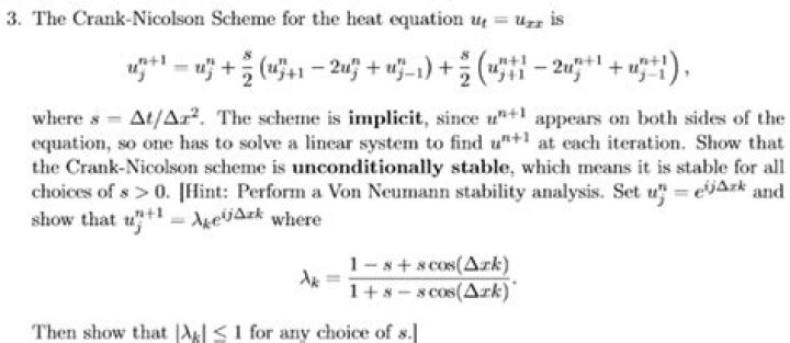
Explanation: When the Crank-Nicolson scheme is applied to the diffusion problems, there is no restriction to the time-step from stability side. It is unconditionally stable for this case. This is why the scheme is often used for diffusion problems.
Is Crank-Nicolson formula converging for all values of λ?
It converges on all values of lambda. When lambda equals to one, that is, k equals to a h squared, the simplest form of the formula is given by value of A which is the average of the values of u at B, C, D, and E.
How stable is the Crank-Nicolson method?
It is a second-order method in time. It is implicit in time and can be written as an implicit Runge–Kutta method, and it is numerically stable. The method was developed by John Crank and Phyllis Nicolson in the mid 20th century. For diffusion equations (and many other equations), it can be shown the Crank–Nicolson method is unconditionally stable.
Does the crank-Nicholson scheme introduce numerical dispersion into the advection problem?
Hence, unlike the Lax scheme, we would not expect the Crank-Nicholson scheme to introduce strong numerical dispersion into the advection problem. Listed below is a routine which solves the 1-d advection equation via the Crank-Nicholson method.
How stable is the Crank-Nicolson method for diffusion equations?
It is implicit in time and can be written as an implicit Runge–Kutta method, and it is numerically stable. The method was developed by John Crank and Phyllis Nicolson in the mid 20th century. For diffusion equations (and many other equations), it can be shown the Crank–Nicolson method is unconditionally stable.
Why is the Crank-Nicolson method more accurate than the backward Euler method?
For this reason, whenever large time steps or high spatial resolution is necessary, the less accurate backward Euler method is often used, which is both stable and immune to oscillations. The Crank–Nicolson method is based on the trapezoidal rule, giving second-order convergence in time.