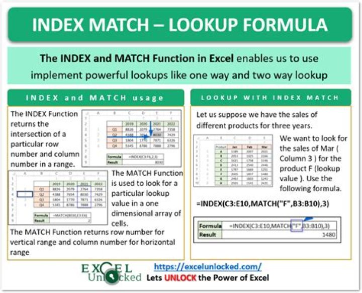
The INDEX function returns a value or the reference to a value from within a table or range. There are two ways to use the INDEX function: If you want to return the value of a specified cell or array of cells, see Array form.
How do I use index function in Excel?
Excel INDEX Function
- Summary. The Excel INDEX function returns the value at a given location in a range or array.
- Get a value in a list or table based on location.
- The value at a given location.
- =INDEX (array, row_num, [col_num], [area_num])
- array – A range of cells, or an array constant.
What is the main function of the index to sheet?
The INDEX function in Google Sheets returns the value of a cell within an input range, relatively separated from the first cell by row and column offsets. This is similar to the index at the end of a book, which provides a quick way to locate specific content.
How do you calculate the index?
The index is calculated by adding the stock prices of the 30 companies and then dividing by the divisor. The divisor changes when there are stock splits or dividends, or when a company is added or removed from the index.
How do you use index formula?
#1 How to Use the INDEX Formula
- Type “=INDEX(” and select the area of the table, then add a comma.
- Type the row number for Kevin, which is “4,” and add a comma.
- Type the column number for Height, which is “2,” and close the bracket.
- The result is “5.8.”
How do I use index function instead of VLOOKUP?
Why use INDEX MATCH instead of VLOOKUP?
- To get the same result using INDEX MATCH, you need to apply the formula =INDEX($C$2:$C$9,MATCH(F2,$A$2:$A$9,0)) to cell G2.
- Using INDEX MATCH will always return the price even after adding/deleting rows as you are using a dynamic reference.
How do you index a list in Excel?
To fetch a certain item from the list, you just write =INDEX(range, n) where range is a range of cells or a named range, and n is the position of the item you want to get.
How do you use an index function in Excel?
Excel INDEX function can be used when you want to fetch the value from a tabular data and you have the row number and column number of the data point. For example, in the example below, you can use the INDEX function to get the marks of ‘Tom’ in Physics when you know the row number and the column number in the data set.
How to create an index formula on Excel?
Type the Name of the item (MacBook) for which price is required in Cell A13. Next, place the curser in Cell B13 and start typing =INDEX – This will bring up the Syntax of Index Function. Select E1:E10 as the INDEX Array – This is where the Price of items is located.
How do you create an index page in Excel?
You can create an index by following the procedure described below: Open your Excel workbook. Insert a new worksheet at the beginning of the workbook. Right click the new worksheet and click Rename. Click the Tools menu, point to Macros, and click Visual Basic Editor. Click Sheet1 (Index) and from the View menu click Code.
What is the most commonly used function in Excel?
The most used functions in Excel are the functions that count and sum. You can count and sum based on one criteria or multiple criteria. To count the number of cells that contain numbers, use the COUNT function. To count cells based on one criteria (for example, greater than 9), use the following COUNTIF function.