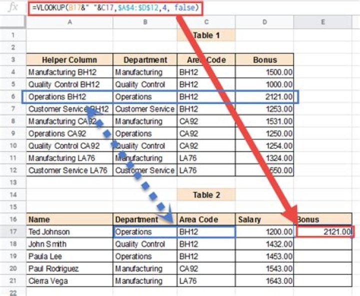
How to Combine VLOOKUP and CHOOSE with Multiple Criteria. A different method to perform the same multiple-criteria lookup is to use a CHOOSE function nested inside your VLOOKUP formula. There are two criteria, the Full Name and the Department, that you can use to get the correct Employee ID.
How do I get rid of Na when using VLOOKUP?
To hide the #N/A error that VLOOKUP throws when it can’t find a value, you can use the IFERROR function to catch the error and return any value you like. When VLOOKUP can’t find a value in a lookup table, it returns the #N/A error.
Can you combine VLOOKUP and if statement in Excel?
One of the most common scenarios when you combine If and Vlookup together is to compare the value returned by Vlookup with a sample value and return Yes / No or True / False as the result. Translated in plain English, the formula instructs Excel to return True if Vlookup is true (i.e. equal to the specified value).
How do you use index and match with multiple criteria?
We use INDEX MATCH with multiple criteria by following these 5 steps:
- Step 1: Understanding the foundation.
- Step 2: Insert a normal MATCH INDEX formula.
- Step 3: Change the lookup value to 1.
- Step 4: Enter the criteria.
- Step 5: Ctrl + Shift + Enter.
Why does my VLOOKUP keep returning na?
The most common cause of the #N/A error is with VLOOKUP, HLOOKUP, LOOKUP, or MATCH functions if a formula can’t find a referenced value. For example, your lookup value doesn’t exist in the source data. In this case there is no “Banana” listed in the lookup table, so VLOOKUP returns a #N/A error.
How do you put 0 instead of #na in Excel?
How to VLOOKUP and return zero instead of #N/A in Excel?
- Select the cell you want to use VLOOKUP function, and type this formula =IFERROR(VLOOKUP(A13,$A$2:$C$10,3,0),0), drag the autofill handle to the range you need.
- Click Kutools > Super LOOKUP > LOOKUP from Right to Left.
How do you do multiple VLOOKUP formulas in Excel?
How to Vlookup and return multiple values in Excel
- Type the formula in the first cell, press Ctrl + Shift + Enter, and then drag it down to a few more cells.
- Select several adjacent cells in a single column (F1:F11 in the screenshot below), type the formula and press Ctrl + Shift + Enter to complete it.
How do you index multiple criteria?
How to use VLOOKUP to return multiple values?
Syntax
How to do multiple vlookups?
If you need to perform multiple lookups sequentially, based on whether the earlier lookups succeed or not, you can chain one or more VLOOKUPs together with IFERROR . The IFERROR function is designed to trap errors and perform an alternate action when an error is detected. The VLOOKUP function will throw an #N/A error when a value isn’t found.
What are the limitations of VLOOKUP?
23 things you should know about VLOOKUP How VLOOKUP works VLOOKUP is a function to lookup up and retrieve data in a table. VLOOKUP only looks right Perhaps the biggest limitation of VLOOKUP is that it can only look to the right to retrieve data. VLOOKUP finds the first match In exact match mode, if a lookup column contains duplicate values, VLOOKUP will match the first value only.
How to count rows based on multiple criteria?
To count rows using multiple criteria across different columns – with OR logic – you can use the SUMPRODUCT function. In the example shown, the formula in H7 is: